학습 및 평가 데이터 분리
from sklearn.model_selection import train_test_split
#출력 데이터 = 의료비,입력데이터 = 그 외 변수
y_column = ['charges']
X = insurance_encoded.drop(y_column, axis=1)
y = insurance_encoded[y_column]
# x,y의 0.2 정도를 평가 데이터로 학습
X_train, X_test, y_train, y_test = train_test_split(X, y,
test_size=0.2,
random_state=42)
특성 스케일링 (권장사항)
서로 다른 수치형 데이터 특성 사이의 값 범위를 비슷하게 맞춰주는 과정
효과: 경사 하강법 사용하는 과정에서 수렴 속도를 높일 수 있음, 일부 특성에 강하게 규제가 걸리는 과정 회피
방법1. StandardScaler
평균 0 표준편차 1로 조정
데이터의 분포가 정규분포일 경우 사용하면 제일 좋음
방법2. MinMaxScaler
최댓값 1, 최솟값 0이 되도록 조정
이상치가 큰 영향을 미치는 경우 사용
출력할 값은 스케일링 하지 않음. 역스케일링 해야하기 때문에 값에 변화가 생길 수 있음
from sklearn.preprocessing import StandardScaler
encoded_columns = list(set(insurance_encoded.columns) - set(insurance_data.columns)) # ['region_southwest', 'region_southeast', 'region_northwest', 'smoker_yes', 'sex_male']
#수치형이었던 데이터 스케일링 해주기
continuous_columns = list(set(insurance_encoded.columns) - set(encoded_columns) - set(y_column)) # ['bmi', 'age', 'children']
scaler = StandardScaler()
# 수치형 데이터만 스케일링 진행
X_train_continuous = scaler.fit_transform(X_train[continuous_columns])
X_test_continuous = scaler.fit_transform(X_test[continuous_columns])
# 스케일 된 데이터와 스케일에 사용되지 않은 데이터 조합
X_train_continuous_df = pd.DataFrame(X_train_continuous, columns=continuous_columns)
X_test_continuous_df = pd.DataFrame(X_test_continuous, columns=continuous_columns)
X_train_categorical_df = X_train[encoded_columns].reset_index(drop=True)
X_test_categorical_df = X_test[encoded_columns].reset_index(drop=True)
X_train_final = pd.concat([X_train_continuous_df, X_train_categorical_df], axis=1)
X_test_final = pd.concat([X_test_continuous_df, X_test_categorical_df], axis=1)
모델 학습하기
from sklearn.linear_model import LinearRegression
# 선형 회귀 모델 초기화 및 학습
linear_reg = LinearRegression()
linear_reg.fit(X_train_final, y_train)
# 학습된 모델의 계수(coefficients) 및 절편(intercept) 출력
coefficients = linear_reg.coef_
intercept = linear_reg.intercept_
print('#'*20, '학습된 파라미터 값', '#'*20)
print(coefficients)
print('#'*20, '학습된 절편 값', '#'*20)
print(intercept)
#################### 학습된 파라미터 값 ####################
[[ 5.16890247e+02 2.03622812e+03 3.61497541e+03 -3.70677326e+02
-6.57864297e+02 2.36511289e+04 -1.85916916e+01 -8.09799354e+02
0.00000000e+00]]
#################### 학습된 절편 값 ####################
[8955.2448015]8개의 특성을 가진 파라미터 값(w1~wn)과 한 개의 학습된 절편(w0) 값 출력
학습 모델 평가 진행 MSE 진행
from sklearn.metrics import mean_squared_error
# 예측 수행
y_train_pred = linear_reg.predict(X_train_final)
y_test_pred = linear_reg.predict(X_test_final)
# 평가 지표 계산: MSE
mse_train = mean_squared_error(y_train, y_train_pred)
mse_test = mean_squared_error(y_test, y_test_pred)
print('학습 데이터를 이용한 MSE 값 :', mse_train)
print('평가 데이터를 이용한 MSE 값 :', mse_test)
학습 데이터를 이용한 MSE 값 : 37277681.70201867
평가 데이터를 이용한 MSE 값 : 33585879.168265626
잘한 걸까? 못한 걸까? 시각화로 확인해보기

선위에 점이 있을수록 예측을 잘 한 것.
그래프 상 x값이 작을수록 결과가 좋음. 점들을 선그래프 위에 위치할 수 있도록 조정해주면서 학습시키기
선형 회귀 모델에 영향을 미치는 변수의 중요도
coeff_df = pd.DataFrame({'feature': X_train_final.columns, 'coefficient': linear_reg.coef_.flatten()})
# 계수의 절대값을 기준으로 내림차순 정렬
coeff_df['abs_coefficient'] = coeff_df['coefficient'].abs()
coeff_df_sorted = coeff_df.sort_values(by='abs_coefficient', ascending=False)
# 변수의 영향력을 확인
coeff_df_sorted
	feature	coefficient	abs_coefficient
5	smoker_yes	23651.128856	23651.128856
2	age	3614.975415	3614.975415
1	bmi	2036.228123	2036.228123
7	region_southwest	-809.799354	809.799354
4	region_southeast	-657.864297	657.864297
0	children	516.890247	516.890247
3	region_northwest	-370.677326	370.677326
6	sex_male	-18.591692	18.591692
8	bias	0.000000	0.000000
abs_coefficient -> 절대값으로 확인해보기

흡연여부가 의료비에 영향을 가장 많이 미치는 것을 알 수 있음
잔차 분석
예측한 값과 정답과의 차이 그래프로 확인해보기
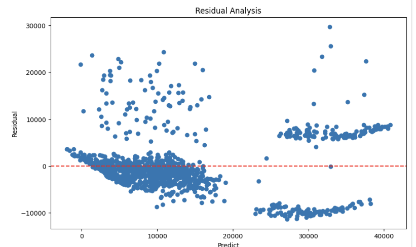
예측값이 작을수록 정답과 가까워짐, 예측값이 크면 잔차가 커지는 특성을 보임
'ML' 카테고리의 다른 글
| [Kaggle] 선형회귀모델학습-의료 보험료 예측하기 |EDA-매트릭스 시각화, 원핫인코딩, 범주형을 수치형으로 변환하기 (0) | 2024.02.01 |
|---|---|
| [ML] 다중공선성 | SVD-OLS | Over fitting | 랏쏘회귀, 릿지회귀 (1) | 2024.02.01 |
| [ML]선형의 의미 | 다중공선성 | 선형 회귀 | 비용 함수 - 정규방정식, 경사 하강법 (0) | 2024.02.01 |
| [ML] 학습,검증,평가 데이터 분할 | overfitting 과적합 | 손실함수 | 파라미터와 최적화 | 분류와 회귀 대표알고리즘 (2) | 2024.01.30 |
| [ML]scikit-learn | Pipeline | 지도학습이란?| 분류와 회귀문제 | 이진분류, 다중클래스 (0) | 2024.01.30 |